Crossfire off South Shore - BOCA race 2015. Yacht navigation requires a good understanding of velocity, distance and time.
|
Projectiles >>
|
1.3 - The Equations of Motion
Objectives:
- To know the three main equations of motion
- To be able to use the equations of motion to solve kinematics problems in one-dimension.
- To be able to demonstrate their accuracy in a practical experiment
There are three basic linking equations between the kinematic variables. Textbooks often have another one or two, but these three will do everything and it is well worth the effort to put them to memory either by learning them rote or just lots of practice. You should be familiar with their derivation although that is not required in the exam.
The first equation should be familiar to you. It is the acceleration and the equation is based on the gradient of the \(v-t\) graph. \[a = \frac{\Delta v}{t}\]
The first equation should be familiar to you. It is the acceleration and the equation is based on the gradient of the \(v-t\) graph. \[a = \frac{\Delta v}{t}\]
The second equation is based on the area under the \(v-t\) graph. Students often struggle with rearranging this equation at first as it almost has everything: we have fractions, addition/subtraction/multiplications and squares. Frequently the initial velocity is set to zero, which simplifies things a great deal. It is a quadratic equation. \[x = v_{o}t +\frac{1}{2}at^{2}\]
The final equation is a very useful one as it does not contain the time variable. We often use this in the lab for calculating the acceleration of a moving object. It is derived by merging the first equation and the average velocity:
\[ a = \frac{(v - v_o)}{t}\]
\[(v-v_o) = at\]
Then the average velocity:
\[\bar{v} = \frac{(v+v_o)}{2}\]
\[\bar{v} = \frac{x}{t}\]
\[t = \frac{x}{\bar{v}} = \frac{2x}{(v+v_o)}\]
Substitute in:
\[(v - v_o) = a \frac{2x}{(v+v_o)}\]
rearrange:
\[(v - v_o) (v+v_o) = 2ax\]
expand out brackets:
\[v^{2}=v_{o}^{2}+2ax\]
With kinematics problems, if you know any three of the five variables, you can calculate the other two. So, the trick is to identify them when you draw the diagram. Some students prefer to list the variables that they know. Although I am not a fan of this practice, it does work well for simple scenarios. Sometimes the variables are not explicitly mentioned in the problem. Look for the clues: At rest or stationary means that the velocity at that point is zero. When an object is thrown into the air, the vertical velocity at the maximum altitude is zero. The acceleration of free fall is \(-g\) - think about the sign. Gravity acts downwards. So objects going upwards (dispacement positive) slow down, while objects moving downwards (displacement negative) speed up. On a practical note, you should also be confident that you can measure each variable in the lab using the most accurate methods available and describe the experiments in detail. Problems at this level often consist of multiple parts - so the variables can 'change' names - e.g. the final velocity of the first part of the motion will become the initial velocity of the second part. At AP or college-level the acceleration for any given segment of an object's motion will be constant.
|
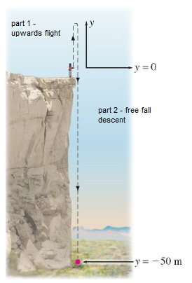
With some of the one-dimensional problems that you have been set in class and for homework you may have to either a) break a scenario into two of more segments or b) be really careful with the signs of the vectors. A classic problem is: you are standing on the edge of a cliff and throw a ball upwards. How fast will it hit the ground? This is best thought of split into TWO parts. Part 1: The flight of the ball upwards from the edge of the cliff to it apex of flight. Part 2: The free fall descent of the ball. However, if you are careful, you can solve the whole problem in one go as the acceleration is constant throughout the scenario. The overall displacement is the height of the cliff downwards, so negative. Whereas the initial velocity is upwards and positive. See below:
|
Example: In the diagram above, the cliff is \(30\,\text{m}\) high and the ball is thrown upwards at \(8\,\text{m/s}\).
Consider the upwards section of the motion. We know the following information; \(v_o=8\,\text{m/s}\), the rate that it decelerates, \(a=-10\,\text{m/s}^2\), and \(v=0\) as it momentarily comes to a stop at the apex of its trajectory. In order to find the height gained we can use
\[v^2 = v_{o}^2+2ax\]
\[0=8^2+(2\times -10 \times x)\]
\[20x = 64\]
\[x=3.2\,\text{m}\]
For the downwards section of the problem, we now effectively have a free fall situation from the height of the cliff plus the height gained from the upwards throw, \(30 + 3.2 = 33.2 \,\text{m}\). This time the ball starts from rest, \(v_o=0\) and the ball accelerates as it falls.
\[v^2 = v_{o}^2+2ax\]
\[v^2 = 0 + (2 \times 10 \times 33.2)\]
\[v^2 = 664\]
\[v= 25.8\,\text{m/s}\]
As the acceleration is constant throughout this scenario - downwards at \(10\,\text{m/s}^2\), we could have also solved in a single step, but we have to be careful with signs. If we set the downwards vectors as negative, we have the following initial information; \(v_o=+8\,\text{m/s}\), \(a= -10\,\text{m/s}^2\) and \(x=-30\,\text{m}\).
\[v^2 = v_{o}^2+2ax\]
\[v^2 = 8^2+(2\times -10 \times -30)\]
\[v^2 = 64 +(600)\]
\[v^2 = 664\]
\[v= 25.8\,\text{m/s}\]
Once the velocity and/or the heights have been calculated, it is possible to calculate the time-of-flight using either of the equations involving \(t\). the easier one is usually \(a=\frac{\Delta v}{t}\) as the other one could end up requiring the quadratic formula to solve if the initial velocity is not zero.
|
More complex problems
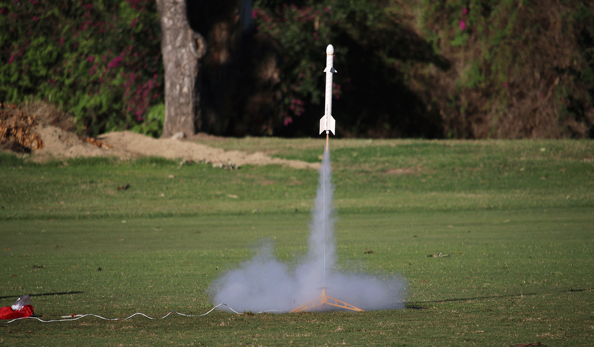
if the acceleration CHANGES during the motion, we must break the motion into sections. It is impossible to solve otherwise. A classic scenario is a rocket that accelerates upwards at \(20\,\text{m/s}^2\) for \(8\,\text{s}\) due to its engine, then once the engine cuts out it coasts to a stop, then falls back to the ground. There are TWO accelerations to consider - the upwards one due to the rocket engine and the downwards pull of gravity. |
Step 1 - Upwards acceleration:
\[a=\frac{(v-v_o)}{t}\]
\[v = v_o+at\]
\[v=0+(20\times8)\]
\[v=160\,\text{m/s}\]
height gained from launch until engine cut off:
\[x=v_ot+\frac{1}{2}at^2\]
\[x=0+\frac{1}{2}\times20\times(8^2)\]
\[x=640\,\text{m}\]
Step 2 - free fall (as previous example, but now the "cliff" is \(640\,\text{m}\) high.
\[v^2 = v_{o}^2+2ax\]
\[v^2 = (160)^2 + (2\times -10 \times -640)\]
TOP TIP - if you find yourself getting caught up in lots of very complicated algebra, STOP. You are probably doing something wrong. There is usually a simpler way of solving it.
Suggested Labs
- Students to find the acceleration of a yoyo as it falls using only meter stick and stopclock. Draw graphs of distance, velocity and acceleration against time.
- A student draws a curvy graph of either x, v or a against time. Another student has to walk according to graph. Other students decide if correct.
- Use the PhysGL software to animate a ball being thrown upwards into the air and falling again.
| lab_1.2_-_animations.pdf |
- Use the equations of motion to determine the acceleration of free fall
| lab_1.4_lab_gravity.docx |
ASSIGNMENTS
| cw_1.3_equations_of_motion_problems.pdf |
| cw_1.4_summary_questions.pdf |
| hw_1.1_acceleration.pdf |
| hw_1.3_froghopper.pdf |
| hw_1.4_up_and_down.pdf |
Projectiles >>
Other Resources
|
Bozeman Science - Motion This is an excellent video that describes position, velocity and acceleration
|
|
Motion Graphs - interactive graphing
|
Wonders of Physics - Kinematics. Excellent cartoons from Evan Toh
|
CK12 Physics - Motion - great site loaded with videos

|
|
Tracker - a computer based version of the VideoPhysics app. A bit more flexible than the app and more accurate as you can import a video from a higher quality camera than the iPad has. The mouse pointer is easier to use! The video tutorial is a bit of a must.
|